Actuarial
  • Research and White Papers
  • September 2023
  • 20 minutes

Multivariable Mortality Modeling, Survival Analysis, and Machine Learning

A pair of African American women review an analysis on a computer.
In Brief

This article from Longevity Bulletin provides an overview of mortality modeling under the survival analysis framework, machine learning methods, extensions to the GLMs, and examples of applying these models. With better predictions and understanding of mortality and longevity risks, (re)insurers and pension funds can leverage these advances to provide financial protection more effectively to more people.

In this article I set out an overview of mortality modeling using survival analysis techniques, a discussion of machine learning methods, extensions to the generalized linear models (GLM), and some examples of applying these models. The focus will be on the use of individual-level data in models that incorporate a multitude of risk factors, rather than group-level or population-level data.

1. Mortality modeling and survival analysis

Traditionally, actuaries and demographers made extensive use of mortality rates, i.e., the probability of a group of similar lives dying in one year. In more recent times, mortality modeling has advanced considerably, with model development employing a statistical framework capable of statistical tests and confidence intervals. At the same time, there has been a significant increase in the volume, veracity, velocity, and variety of data available for analysis, which encompasses policyholder data, demography, postcodes, electronic health records, lifestyle, and credit scores.

As insurers and pension schemes collect experience data on individual policyholders, this is essentially a form of longitudinal study because the individuals are observed for a period of time until a particular event of interest occurs (known as time-to-event or survival time).

The main challenge of time-to-event data is the presence of incomplete observations. This occurs due to censoring, i.e., when a death event happens outside of the observation period. For this reason, many classical statistical models and machine learning methods could not transpose directly to time-to-event data.

Modeling time-to-event data requires a specific approach called survival analysis. It is used to predict the target variable of survival time until mortality, while accounting for censoring, and the presence of explanatory variables that may affect survival time (Rodríguez, 2007).

Survival analysis is a very useful tool in evaluating risks such as mortality, longevity, morbidity, lapses, and demographic factors (e.g., marriage, migration, and fertility). As the name indicates, survival analysis has origins in the field of medical research to estimate the survival rate of patients after a medical treatment. It is also known as reliability analysis in engineering, duration analysis in economics, and event history analysis in sociology (Abbas et al., 2019).

Figure 1 shows a taxonomy of survival analysis models, which provides a holistic view of statistical and machine learning methods, categorized by continuous-time and discrete-time approaches (with separate charts for each).

Figure 1

1.1 Continuous-time survival analysis

Survival analysis theory focuses on two key concepts in continuous time:

a. the survival function S(t), i.e., the probability of being alive just before duration t

b. the hazard function h(t), i.e., the instantaneous death rate at time t, also known as the force of mortality by actuaries

There is a one-to-one relationship between the hazard function and the survival function. Whatever functional form is chosen for the hazard function, one could use it to derive the survival function. The integral of the survival function then gives the expectation of life, i.e., mean of survival time (Rodríguez, 2007).

1.1.1 Non-parametric models

The non-parametric methods are simple and require no assumptions on distributions. The Kaplan-Meier estimator, also known as the product limit estimator, provides an empirical estimate of the survival function. The Nelson- Aalen estimator approximates the cumulative hazard function. As the sample size gets very large, these two estimators are asymptotically equivalent (Jenkins, 2005). Kaplan-Meier and Nelson-Aalen are univariable methods and likely to be less predictive; therefore, considering multivariable methods is recommended if multiple explanatory variables are available.

1.1.2 Semi-parametric models

In the semi-parametric category, the Cox proportional hazard model was proposed by Cox (1972) in perhaps the most often cited article on survival analysis. The hallmark of the Cox model is that it allows one to estimate the relationship between the hazard function and explanatory variables, without having to make any assumption on the baseline hazard function. Proportional hazards modeling assumes that the ratio of the hazards for any two individuals is constant over time. The fact that the hazards are proportional is helpful in making interpretations, such as when identifying the better treatment in medical trials or analyzing loadings of risk factors in underwriting. The Cox model can also be generalized to handle time-varying covariates and time-dependent effects (Rodríguez, 2007).

The Piecewise-Constant Exponential (PCE) model is another example of semi-parametric continuous-time model and can be seen as a special type of proportional hazards model (Jenkins, 2005). When the time axis is partitioned into a number of intervals in a PCE model, it assumes that the baseline hazard is constant within each interval. The advantage is that one does not have to impose the overall shape of the hazard function in advance. Another useful property of the PCE model is its equivalence to a certain Poisson GLM model; this will be discussed later.

1.1.3 Parametric models

Parametric statistical methods assume that survival time follows a particular theoretical distribution (Wang et al., 2019). Commonly used distributions include exponential, Weibull, Normal, Gamma, log-logistic, log-normal, and Gompertz (Jenkins, 2005). If the survival time follows the assumed distribution, resulting outcomes are accurate, efficient, and easy to interpret, but if the assumption is violated parametric models can give sub-optimal results.

Another approach in the parametric category is the accelerated failure time (AFT) model. AFT assumes a linear relationship between the log of survival time and the explanatory variables. The effect of variables is to accelerate or decelerate the life course. The Weibull model is the only model that satisfies both proportional hazards and AFT assumptions (Rodríguez, 2007).

1.1.4 Other continuous-time models

As discussed in Bayesian Survival Analysis (Ibrahim et al., 2001), Bayesian approaches can be applied to survival models, including parametric, proportional, and non-proportional models. Interpretability is a strength of Bayesian modeling. Other examples of survival models include machine learning methods, which will be discussed in Section 2, as well as competing-risk and multi-state models (Jenkins, 2005).

1.2 Discrete-time survival analysis

The survival analysis techniques discussed in the previous section assume continuous measurement of time. Although it is natural to consider time as a continuous variable, in practice observations are often on a discrete time scale, such as days, months or years (Jenkins, 2007). An advantage of discrete-time modeling is the embedding of the GLM framework.

Interestingly, the PCE model is equivalent to a GLM Poisson log-linear model for discretized pseudo-data, when the death indicator is the response, and the log of exposure times is the offset (Rodríguez, 2007). The likelihood function of PCE and independent Poisson observations happen to coincide and would therefore lead to the same estimates.

Generally, the choice of GLM for survival analysis depends on the nature of data (Rodríguez, 2007):

i. If data is continuous and if one is willing to assume hazard is constant in each interval, the Poisson GLM is appropriate as it allows use of partial exposures

ii. If data is truly discrete, logistic regression is recommended

iii. If data is continuous but only observed in grouped form, the complementary log-log link is preferable.

View other issues of the IFoA’s Longevity Bulletin.

2. Machine learning models for survival analysis


In recent years, machine learning models have achieved success in many areas. This is due to built-in strengths that include higher prediction accuracy, ability to model non-linear relationships, and less dependence on distribution assumptions. Nevertheless, some machine learning algorithms bring notable weaknesses as well, such as difficulty in interpretation, sensitivity to hyperparameters, and a tendency to overfit. Dealing with censored data presents the biggest challenge for using machine learning in survival analysis.

A deeper understanding of survival analysis, and how machine learning can overcome the challenge of censored data, is required in order to effectively adapt it to mortality modeling.

The discussion below starts with regularization – a versatile machine learning technique applicable to many approaches, including GLM and classical survival models. The total range of machine learning models is vast; therefore, I look just at continuous-time models and deliberately exclude some notable discrete-time approaches, for instance support vector machines and random forest. Discrete-time supervised machine learning models are discussed in Modeling Discrete Time to Event Data (Tutz and Schmid, 2018), while extensions of GLM are discussed in Section 3.

2.1 Regularization

Regularization is a technique used to simplify a model and reduce overfitting by adding penalties or constraints to the model-fitting problem. The three main types of regularization are:

i. Ridge, also known as Tikhonov or L2 regularization, adds a penalty term based on the squared value of coefficients. It reduces the size of coefficients and deals with correlations between features simultaneously.

ii. Lasso (least absolute shrinkage and selection operator), also known as L1 regularization, adds a penalty term based on the absolute value of coefficients. In contrast to Ridge, Lasso can shrink coefficients to zero, which means it can perform automatic variable selection. Extensions of Lasso include Group Lasso, Fused Lasso, Adaptive Lasso, and Prior Lasso.

iii. Elastic net linearly combines the Ridge and Lasso penalty terms.

2.2 Cox models

Introducing regularization into Cox proportional hazard models provides us with a form of machine learning – the resulting models include Ridge-Cox (Verweji and Van Houwelingen, 1994), Lasso-Cox (Tibshirani, 1997), and Elastic Net-Cox (Simon et al., 2011).

The Cox-Boost method (Binder and Schumacher, 2008) incorporates gradient boosting machines in Cox models. It is useful on high-dimensional data and considers some mandatory variables explicitly in the model.

2.3 Survival tree

Survival trees are classification and regression trees (CART) specifically designed to handle censored data (Gordon and Olshen, 1985). The data is recursively partitioned based on a splitting criterion and objects with similar survival times are grouped together. This approach is easier to interpret and does not rely on distribution assumptions.

2.4 Random survival forest and other ensemble methods

In machine learning, ensemble learning is a method that takes a weighted vote from multiple models to obtain better predictive performance than could be obtained from any of the constituent models alone. Common types of ensembles include bagging, boosting, and stacking.

Bagging survival trees involves taking a number of bootstrap samples from the survival data, building a survival tree for each sample, and then averaging the tree nodes’ predictions (Hothorn et al., 2004).

Random survival forest is similar to bagging, but random forest uses only a random subset of the features for selection at each tree node. This helps reduce the correlation between trees and improves predictions. Random survival forest does not depend on distribution assumptions and can be used to avoid the proportional hazards constraint of a Cox model (Ishwaran et al., 2008).

Boosting combines a set of simple models into a weighted sum and is iteratively fitted to the residuals based on the gradient descent algorithm. Hothorn et al. (2006) proposed gradient boosting to account for censored data.

Stacking combines the output of multiple survival models and runs it through another model. Wey et al. (2015) proposed a framework of stacked survival models that combines parametric, semi-parametric and non-parametric survival models. This approach has performed well by adaptively balancing the strengths and weaknesses of individual survival models.

2.5 Artificial neural networks

Artificial neural networks (ANN) consist of layers of neurons interconnected as a network to solve optimization problems. The adjective ‘deep’ in deep learning refers to the use of multiple layers in the network. Neural networks and survival forests are examples of non-linear survival methods.

The initial adaptation of survival analysis to neural networks sought to generalize Cox with only one single hidden layer (Farragi and Simon, 1995). Katzman et al. (2018) later proposed DeepSurv, a deep feed-forward neural network generalizing the Cox proportional hazards model. It has the advantage of not requiring a priori selection of covariates, by learning them adaptively.

DeepHit is a deep neural network that learns the distribution of survival times directly (Lee et al., 2018). Unlike parametric approaches, it makes no assumption of the underlying stochastic processes and allows for the relationship between covariates and risk to change over time. DeepHit can be used for survival datasets with a single mortality risk as well as multiple competing risks.

3. Extensions and enhancements of GLM

GLM is a popular tool in survival analysis due to its versatility, interpretability, predictive power, and availability in many software packages. Section 1 demonstrated that GLM Poisson, Logistic and C-Log-Log models can perform survival analysis. However, GLMs elicit two common negative views: they are restricted by distribution assumption, and they do not account for non-linear relationships, which reduces predictive performance.

The first view is refutable because, as discussed in Section 1, a GLM is merely a device to derive the underlying survival model, so the model is not restricted by distribution assumptions of GLM.

The second issue can be mitigated using approaches such as these to extend or enhance GLM. Note that these are not restricted to survival analysis and can be applied to GLMs in general. Some practitioners would view these as ways to combine the advantages of GLMs (for instance, interpretability) with the power of machine learning:

  1. Generalized additive model (GAM): GAM is a GLM in which one or more of the predictors depends linearly on some smooth functions, which is useful to capture non-linear patterns. Examples of smooth functions are cubic splines and fractional polynomials. This approach allows much more flexible models.
  2. Generalized linear mixed model (GLMM): The GLMM extends the GLM by incorporating random effect terms. GLMMs are also referred to as frailty models (Tutz and Schmid, 2018).
  3. Regularization such as elastic net to handle multicollinearity and reduce overfitting.
  4. Automatic variable selection using Lasso or elastic net. This can help identify influential risk factors efficiently rather than using stepwise selection, especially when the number of possible predictors is large.
  5. Identification of predictive interaction terms with the help of machine learning, such as decision trees or random forest. If interpretability is important, it is preferable to keep the interaction terms relatively simple, rather than incorporating an influential yet hard-to-interpret ‘blackbox’ sub-model, such as a neural network, into a GLM.
  6. Dimension reduction, by using unsupervised machine learning techniques, if there is a very large number of variables relative to the number of observations.

4. Applications in mortality modeling

Tedesco et al. (2021) constructed machine learning models to predict all-cause mortality in a two- to seven-year time frame in a cohort of healthy older adults. The models were built on features including anthropometric variables, physical and lab examinations, questionnaires, and lifestyle factors, as well as wearable data. Random forest showed the best performance, followed by logistic regression, AdaBoost, and decision tree. Additional insights could be extracted to gain understanding on healthy aging and long-term care.

Using the MIMIC-III dataset on long-term mortality after cardiac surgery and the AUC metric, the researchers observed the order of model performance, from highest to lowest, to be AdaBoost, logistic regression, neural network, random forest, Naïve Bayes, XGBoost, bagged trees and gradient-boosting machine (Yu et al., 2022).

The OpenSAFELY paper (Williamson, 2020) applied the multivariable Cox model to analyze data from 17 million patients in England and subsequently identified a range of risk factors for Covid-19 mortality This was instrumental in helping to identify high-risk population subgroups, as Dan Ryan describes elsewhere in this Bulletin. Later that year, RGA (Ng et al., 2020) published a paper that cross-compared an all-cause mortality model with OpenSAFELY’s Covid-19 model in a parallel and multivariable way. This revealed insights on excess mortality risk from certain factors, which were useful to actuaries and underwriters. Six months later, the OpenSAFELY team published another paper (Bhaskaran et al., 2021) analyzing Covid-19 and non-Covid-19 mortality odds ratios, by using logistic regression. The team produced results that were very consistent with RGA’s.

Conclusion

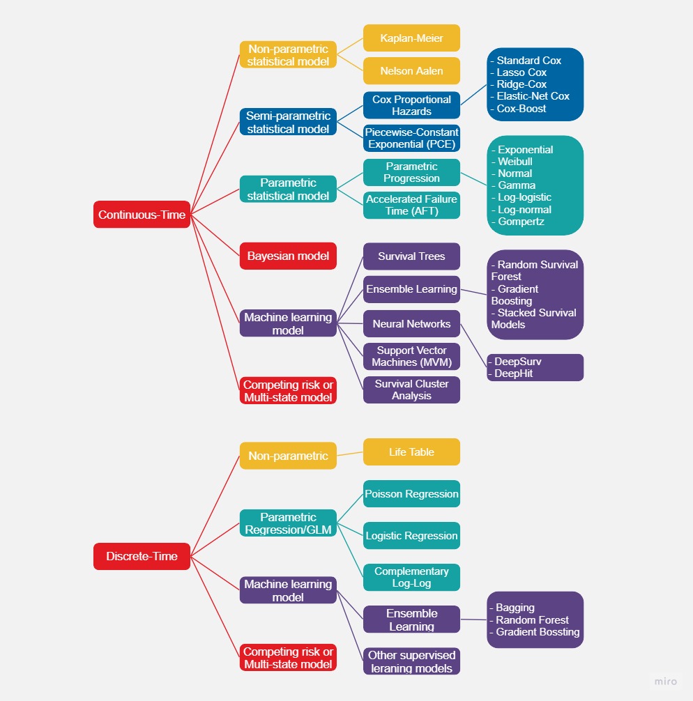
The goal of mortality modeling is to predict and understand mortality and longevity. This article provides a survey and taxonomy of mortality modeling under the survival analysis framework, structured by continuous-time and discrete-time, as well as statistical methods and machine learning. The choice of model depends on the nature of the data and the purpose – whether it is solely about predictive accuracy or if interpretability is important.

Due to the increasing availability of data, technology and development in survival analysis and machine learning, financial services providers, such as insurers and pension funds, can leverage advances in these areas to provide financial protection more effectively to more people.


Reprinted with permission of The Institute and Faculty of Actuaries.

Watch the recording of this topic as part of the IFoA Longevity and Mortality webinar series.

More Like This...

Meet the Authors & Experts

John Ng
Author
John Ng
Director, Longevity Analytics, Global Financial Solutions

References

    Abbas, S.A., Subramanian, S., Ravi, R., et al. (2019). An introduction to survival analytics, types, and its applications. https://www.intechopen.com/chapters/64244 [Accessed 2 Feb 2023.]

    Bhaskaran, K., Bacon, S., Evans, S.J.W., et al. (2021). Factors associated with deaths due to COVID-19 versus other causes: population-based cohort analysis of UK primary care data and linked national death registrations within the OpenSAFELY platform. The Lancet Regional Health - Europe, 6: 100109. https://doi.org/10.1016/j.lanepe.2021.100109

    Binder, H. and Schumacher, M. (2008). Allowing for mandatory covariates in boosting estimation of sparse high-dimensional survival models. BMC Bioinformatics, 9. https://doi.org/10.1186/1471-2105-9-14

    Cox, D.R. (1972). Regression models and life-tables. Journal of the Royal Statistical Society. Series B (Methodological), 34(2): 187-220. http://www.jstor.org/stable/2985181

    Faraggi, D. and Simon, R. (1995). A neural network model for survival data. Statistics in Medicine, 14(1): 73-82. https://doi.org/10.1002/sim.4780140108

    Gordon, L. and Olshen, R.A. (1985). Tree-structured survival analysis. Cancer Treatment Reports, 69(10): 1065-9.

    Hothorn, T., Lausen, B., Benner, A., et al. (2004). Bagging survival trees. Statistics in Medicine, 23(1): 77-91. https://doi.org/10.1002/sim.1593

    Hothorn, T., Buhlmann, P., Dudoit, S., et al. (2006). Survival ensembles. Biostatistics, 7(3): 355-373. https://doi.org/10.1093/biostatistics/kxj011

    Ibrahim, J.G., Chen, M.H. and Sinha, D. (2001). Bayesian survival analysis. New York: Springer.

    Ishwaran, H., Kogalur, U.B., Blackstone, E.H., et al. (2008). Random survival forests. Annals of Applied Statistics, 2(3): 841-860. https://doi.org/10.1214/08-AOAS169

    Jenkins, S.P. (2005). Survival analysis. https://www.iser.essex.ac.uk/files/teaching/stephenj/ec968/  pdfs/ec968lnotesv6.pdf [Accessed 2 Feb 2023.]

    Katzman, J.L., Shaham, U., Cloninger, A., et al. (2018). DeepSurv: personalized treatment recommender system using a Cox proportional hazards deep neural network. BMC Medical Research Methodology, 18. https://doi.org/10.1186/s12874-018-0482-1

    Lee, C., Zame, W.R., Yoon, J. et al. (2018). DeepHit: A deep learning approach to survival analysis with competing risks. Proceedings of the AAAI Conference on Artificial Intelligence, 32(1). https://doi.org/10.1609/aaai.v32i1.11842

    Ng, J., Bakrania, K., Falkous, C., et al. (2020). COVID-19 mortality by age, gender, ethnicity, obesity, and other risk factors: a comparison against all-cause mortality.

    RGA, 18 December. https://www.rgare.com/knowledge-center/ media/research/covid-19-mortality-by-age-gender-ethnicity- obesity-and-other-risk-factors [Accessed 2 Feb 2023.]

    Rodríguez, G. (2007). Lecture notes on generalized linear models. https://grodri.github.io/glms/notes/ [Accessed 18 July 2023.]

    Simon, N., Friedman, J., Hastie, T., et al. (2011). Regularization paths for Cox’s proportional hazards model via coordinate descent. Journal of Statistical Software, 39(5): 1-13. https://doi.org/10.18637/jss.v039.i05

    Tedesco, S., Andrulli, M., Larsson M.A., et al. (2021). Comparison of machine learning techniques for mortality prediction in a prospective cohort of older adults. International Journal of Environmental Research and Public Health, 18(23): 12806. https://doi.org/10.3390/ijerph182312806

    Tibshirani, R. (1997). The Lasso method for variable selection in the Cox model. Statistics in Medicine, 16(4): 385-395. https://doi.org/10.1002/(sici)1097-0258(19970228)  16:4%3C385::aid-sim380%3E3.0.co;2-3

    Tutz, G. and Schmid, M. (2016). Modeling discrete time-to-event data. New York: Springer.

    Verweji, P.L. and Van Houwelingen, H.V. (1994). Penalized likelihood in Cox regression. Statistics in Medicine, 13(23-24):  2427-36.  https://doi.org/10.1002/sim.4780132307

    Wang, P., Li, Y. and Reddy, C.K. (2019). Machine learning for survival analysis: a survey. ACM Computing Surveys, 51(6). https://doi.org/10.1145/3214306

    Wey, A., Connett, J. and Rudser, K. (2015). Combining parametric, semi-parametric, and non-parametric survival models with stacked survival models. Biostatistics, 16(3): 537-49. https://doi.org/10.1093/biostatistics/kxv001

    Williamson, E.J., Walker, A.J., Bhaskaran, K., et al. (2020). Factors associated with COVID-19-related-death using OpenSAFELY. Nature, 584: 430-6. https://doi.org/10.1038/s41586-020-2521-4

    Yu, Y., Peng, C., Zhang, Z., et al. (2022). Machine learning methods for predicting long-term mortality in patients after cardiac surgery. Frontiers in Cardiovascular Medicine, 9. https://doi.org/10.3389/fcvm.2022.831390