Multi-state models (MSMs) can be used to characterize the transitions of a group of individuals through a succession of states until they reach a particular endpoint known as an “absorbing state”
MSMs are now proving to be particularly popular in medical research, as attention is shifting from studying a single trajectory between two states (such as alive to dead or diseased to dead) to describing entire disease pathways. Modeling trajectories between different disease states, while accounting for competing events at each transition, provides a much clearer understanding of the importance of different risk factors at each transition. As a result, multi-state modeling is a powerful tool to study morbidity and mortality pathways simultaneously – providing valuable knowledge for actuaries and underwriters. Although MSMs are not new in the (re)insurance industry, some recent novel developments have likely yet to be widely adopted by actuaries and data scientists.
Introduction and Example
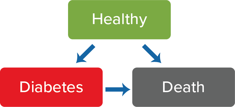
A multi-state model (MSM) allows for the simultaneous estimation of morbidity and mortality risks; therefore, it can be used to analyze a system where individuals transition from one disease state to the next until death (i.e., enter the absorbing state)1,2,3. For example, a typical survival model can be thought of as a straightforward MSM with one transition between two states (alive → dead). In reality, however, an individual may experience a wide range of intermediary morbidity outcomes, such as cancer, myocardial infarction, stroke, and many others. To demonstrate the structure of a simple three-state MSM, consider the states (boxes) and transitions (arrows) in Figure 1 below.
Figure 1:
Figure 2 below demonstrates the corresponding transition matrix (shaded in gray) for this three-state MSM. The column and row numbers are indexed as the states, and the elements are equal to the transition numbers. Any transitions labelled with a dash (–) imply that the progression between the row state and the column state is not allowed. Although this matrix does not allow for any reverse transitions (e.g., diabetes → healthy), they can be included if desired.
Figure 2:
Corresponding transition matrix
Transition Matrix | Healthy | Diabetes | Death |
Healthy | – | 1 | 2 |
Diabetes | – | – | 3 |
Death | – | – | – |
State 1 is a “healthy” state and individuals can start in this state and potentially transition to state 2 (diabetes) or state 3 (death). “Diabetes” is an intermediary state and individuals can start in this state (i.e., prevalent diabetes) or enter it from the “healthy” state (i.e., incident diabetes), and potentially transition to the “death” state. “Death” is the absorbing state and individuals can enter it from the “healthy” state or the “diabetes” state but cannot exit this state. To summarize, the matrix has the following three transitions:
- Transition 1: state 1 → state 2 (i.e., healthy → diabetes)
- Transition 2: state 1 → state 3 (i.e., healthy → death)
- Transition 3: state 2 → state 3 (i.e., diabetes → death)
In medical research, the Cox proportional hazards model is frequently used for the analysis of time-to-event data and could be used to model any of the three transitions above. Although the model is useful for comparing the risk between two groups, it is limited to estimating hazard ratios without approximating the baseline hazard function itself1,2,3. The baseline hazard function is of course of key interest for (re)insurance applications since it represents the change in risk over the timescale of interest (e.g., age or duration since policy inception). The optimal approach for the analysis of survival data would be to use the baseline hazard function for the continuous mathematical estimation of the absolute measures of effect, and in contrast to Cox models, parametric survival models can quantify this function because an underlying distribution (i.e., time-dependency) is specified mathematically2.
Parametric survival models specify the baseline hazard function, and a common specification is the Weibull distribution. In situations where the underlying hazard rate (i.e., the way it changes with the timescale of interest) is monotonically increasing, monotonically decreasing, or constant, the Weibull distribution can provide accurate predictions for absolute measures of effect, and parameter estimates will typically be more precise than estimates from semi-parametric and non-parametric models where the underlying distribution is left unspecified. However, when the hazard function has a more complicated shape, such as decreasing with time in a complex way, specifying a Weibull distribution could lead to inaccurate predictions and/or model convergence issues2. For example, Figure 3 below shows the risk of death following an incident of stroke; initially the risk is very high but decreases thereafter, before increasing again with age.
Figure 3:
Risk of death following an incident of stroke
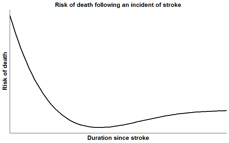
Consequently, although parametric survival models potentially offer smooth predictions via assuming a functional form of the hazard, the assumed form is often too restrictive for use with real data, particularly if there are substantial changes in the shape of the hazard over time. Therefore, a middle ground between the Cox model and the parametric model is required. This is where the flexible parametric survival model comes in, which preserves the desired traits of both models2.
A competing risk is an event that prevents the occurrence of the primary event of interest3,4,5. For example, in a study investigating the time to death attributable to cancer causes, death attributable to non-cancer causes is a competing risk. In essence, MSMs are a harmonization of competing risks models and can be derived by the amalgamation of transition-specific survival models. Accordingly, the three transitions listed earlier define that three-state MSM. Note: Each of these survival models can be as complex as needed. In any scenario, interpretable measures of absolute risk can be obtained. For example, each transition-specific model could have a different:
- distributional family: exponential, Cox model, generalized gamma, Gaussian, Gompertz, general log cumulative hazard model, general log hazard model, log logistic, log normal, piecewise-exponential, Royston-Parmar model on the log cumulative hazard scale, Weibull, and any others
- number of timescales: MSMs can incorporate multiple timescales of age, calendar time, and duration since diagnosis
- covariate pattern: with a variety of different interactions and time-varying effects
For example, the example three-state MSM could have the following:
- Transition 1: healthy → diabetes
- piecewise-exponential distributional family
- single timescale (delayed-entry age: e.g., Person A enters the study at age 47 and develops diabetes at age 50)
- adjusted for gender and smoker status
- Transition 2: healthy → death
- Royston-Parmar model on the log cumulative hazard scale
- single timescale (delayed-entry age: e.g., Person B enters the study at age 37 and dies at age 39)
- adjusted for gender and smoker status
- Transition 3: diabetes → death
- piecewise-exponential distributional family
- multiple timescales (delayed-entry age and delayed-entry duration since diagnosis of diabetes: e.g., Person A developed diabetes at age 50 but the risk of death is studied on the age scale as well as on the duration since diabetes diagnosis scale) *
- adjusted for gender, smoker status, and treatment (one of the big benefits of employing MSMs: each transition can have a different set of risk variables)
* MSMs are usually fitted assuming the Markov assumption, i.e., future transitions depend only on the current state, not on the events that occurred before it2. This can be considered to be restrictive; however, it can be relaxed by allowing the transition intensities to depend on the time at which earlier states were entered, i.e., multiple timescales3,6. Here, on the additional timescale (delayed-entry duration since diagnosis), incident diabetics could enter at time 0 (the clock is reset to 0 for any diabetes incidents observed in transition 1), and prevalent diabetics could enter at time > 0 (a delayed entry); hence, taking any period of immortality into account.
Note: In order to provide a forward-looking view of any future improvements, comprehensive and diverse expert judgement can also be captured for each transition with separate assumptions for each morbidity and mortality model, allowing the researcher to understand the impact on the transition probabilities over time.
Once a series of transition-specific models has been developed, transition probabilities can be computed for any covariate pattern of interest. Point estimates would first be calculated by simulating individuals through the trajectories defined in the transition matrix. Then, at each specified time point, the number of individuals in each state would be counted and divided by the total to obtain the transition probabilities. Other metrics such as the hazard function, survival function, and length of stay in each state can also be computed.
Simulated using dummy data, typical transitions for the simple three-state MSM example in 1,000 individuals may look like those shown in Figure 4 below:
Applications
MSMs are increasingly being used to model intricate disease profiles as they provide a flexible framework for analyzing complex clinical transitions over time. This means that they have great applications in the (re)insurance industry. Some potential use cases include:
- Setting forward-looking all-cause mortality trends by incorporating expert medical judgement
- This can be achieved by using the MSM output (e.g., transitional probabilities) after incorporating expert judgement as to how each transition probability may develop in the future.
- Such an approach ‘builds in’ consistency between morbidity and mortality trends.
- Pricing multi-pay critical illness products
- An MSM facilitates the pricing of products for which individuals receive a partial payout at each transition (e.g., 25% of the face value on diagnosis of cancer in year four, another 25% on diagnosis of a heart attack in year seven, and the remaining 50% on death in year 12). *
- Investigating risk factors and morbidity pathways for underwriting
* Generated using dummy data, a typical payout versus time plot for a multi-pay critical illness product may look like the one shown in Figure 5 below:
Figure 5:
Payout vs. time
There are many other use cases for MSMs in actuarial modeling. This paper has demonstrated some of the advantages of employing MSMs to simultaneously analyze morbidity and mortality outcomes in favor of the more traditional approaches of utilizing survival and longitudinal models.